---
format:
    revealjs:
        logo: img/https___comm.mitre.org_strategiccommunications_wp-content_uploads_sites_170_2020_01_MITRE_logos_Base.svg
        footer: © 2023 THE MITRE CORPORATION. ALL RIGHTS RESERVED. Approved for public release; distribution unlimited. Case number 23-03859-1.
        theme: mitre-template.scss
        width: 1350
        self-contained: true
        preload-iframes: true
        preview-links: true
        disable-layout: false
        code-fold: show
        code-overflow: wrap
        code-copy: hover
        output-location: column
        scrollable: true

---
# Working with Messy Data

<span id="name">Christopher Teixeira</span><br>
`r format(Sys.Date(), "%B %d, %Y")`

::: {.footer id="release-clause"}
The author's affiliation with The MITRE Corporation is provided for identification pusposes only, and is not intended to convey or imply MITRE's concurrence with, or support for, the positions, opinions or viewpoints expressed by the author. 
:::

## A little about me... {.smaller}

<br><br>

:::: {.columns}

::: {.column width="70%"}
<br>

### Christopher Teixeira {id="name"}
### Principal Data Scientist
### The MITRE Corporation

<br><br>

::::{.columns}
::: {.column width="45%"}
#### Interests

- Data Analytics
- Applied Statistics
- Operations Research

:::

::: {.column width="45%"}
#### Education

- MS in Operations Research, George Mason University
- BSc in Mathematics, Worcester Polytechnic Institute

:::
::::

:::

::: {.column width="30%"}

![](img/profile.png){fig-align="center"}

:::
::::

## Setup {visibility="hidden"}

```{r}
#| label: r_setup

library(tidyverse)
library(jsonlite)
library(ggplot2)
library(ggExtra)
library(knitr)
library(scales)

# Practioner data from:
# https://data.cms.gov/provider-summary-by-type-of-service/medicare-physician-other-practitioners/medicare-physician-other-practitioners-by-provider
```

```{python}
#| python.reticulate: FALSE
#| label: python_setup
#| eval: false

# import pandas as pd
# url = "https://data.cms.gov/data-api/v1/dataset/8889d81e-2ee7-448f-8713-f071038289b5/data?size=5000"
# df = pd.read_json(url)
# df.to_html()

# cols = [1,13,20,21,42,43,44,45,46,47,48,49,50,51,52,53,54,55,56,57,58,59,60,61,62,63,64,65,66,67,68,69,70,71,72,73]
# df.loc[:,cols]
# numeric_cols = df.columns.drop(["Rndrng_NPI","Rndrng_Prvdr_Zip5"])
# df[numeric_cols]=df[numeric_cols].apply(pd.to_numeric, errors='coerce')
# categorical_cols = ["Rndrng_NPI","Rndrng_Prvdr_Zip5"]
# df[categorical_cols]=df[categorical_cols].apply(pd.Categorical)

```

## Reading in data {.smaller}

::: {.panel-tabset}

### R

```{r}
#| label: r_readdata
#| echo: true

# URL for the CMS data used in these slides
url <- "https://data.cms.gov/data-api/v1/dataset/8889d81e-2ee7-448f-8713-f071038289b5/data?size=5000"

# Download and convert the JSON file to a data frame
df <- jsonlite::fromJSON(url)

# View the data frame in a friendly format for Quarto
knitr::kable(head(df), format="html")

```

### Python

```{python}
#| label: python_readdata
#| python.reticulate: FALSE
#| eval: false
#| echo: true

import pandas as pd

# URL for the CMS data used in these slides
url = "https://data.cms.gov/data-api/v1/dataset/8889d81e-2ee7-448f-8713-f071038289b5/data?size=5000"

# Download and convert the JSON file to a data frame
df = pd.read_json(url)

# View the data frame in a friendly format for Quarto
df.to_html()

``` 

:::

## Changing data types {.smaller}

::: {.panel-tabset}

### R

```{r}
#| label: r_datatypes
#| echo: true

# Subset the data down to a select few to work with. 
# Then convert "Bene_" and "Tot_" variables to numeric. 
# The ID and zip code variables get converted to factors.
df.subset <- df |> 
    select(Rndrng_NPI,
           Rndrng_Prvdr_Zip5,
           Tot_Benes,
           Tot_Srvcs,
           starts_with("Bene_")) |>
    mutate(across(starts_with(c("Bene_","Tot_")), as.numeric),
           across(starts_with("Rndrng_"), factor))

# View the data frame in a friendly format for Quarto
knitr::kable(head(df.subset), format="html")
```

### Python

```{python}
#| label: python_datatypes
#| python.reticulate: FALSE
#| eval: false
#| echo: true

# Subset down to the columns of interest.
cols = [0,12,19,20,41,42,43,44,45,46,47,48,49,50,51,52,53,54,55,56,57,58,59,60,61,62,63,64,65,66,67,68,69,70,71,72]
df_subset = df.iloc[:,cols]

# Convert character to numeric columns. 
numeric_cols = df_subset.columns.drop(["Rndrng_NPI","Rndrng_Prvdr_Zip5"])
df_subset[numeric_cols]=df_subset[numeric_cols].apply(pd.to_numeric, errors='coerce')

# Convert ID and zip code columns to categorical. 
categorical_cols = ["Rndrng_NPI","Rndrng_Prvdr_Zip5"]
df_subset[categorical_cols]=df_subset[categorical_cols].apply(pd.Categorical)

```

:::

## Exploratory data analysis {.smaller}

Exploratory data analysis (EDA) is used by data scientists to analyze and investigate data sets and summarize their main characteristics, often employing data visualization methods. It helps determine how best to manipulate data sources to get the answers you need, making it easier for data scientists to discover patterns, spot anomalies, test a hypothesis, or check assumptions. ^[[IBM What is exploratory data analysis?](https://www.ibm.com/topics/exploratory-data-analysis)]

<br><br>

Four primary types of EDA:

1. **Univariate non-graphical**: Describe the data and find patterns that exist within a variable.
2. **Univariate graphical**: For a single variable, explore the values visaully using graphs like box plots or histograms.
3. **Multivariate nongraphical**: Describe the relationships between two or more variables in the data. 
4. **Multivariate graphical**: Visualize the relationships between two or more variables through graphs like scatter plots or heat maps, 

## Applying EDA: Univariate {.smaller}

::: {.panel-tabset}

### R

```{r}
#| label: r_eda_univariate
#| echo: true

# Use the skimr package to examine the dataset. 
# Produces a high level summary (# of rows/columns, column types)
# For each column type, it produces details about each variable.

library(skimr)
skim(df.subset)

```

### Python

```{python}
#| label: python_eda_univariate
#| python.reticulate: FALSE
#| eval: false

from pyskim import skim
skim(df_subset)

```

:::

## Applying EDA: Multivariate {.smaller}

::: {.panel-tabset}

### R

```{r}
#| label: r_eda_multivariate
#| echo: true
#| fig-height: 7

library(ggplot2)
library(ggExtra)
library(ggthemes)

# Create a scatter plot with the number of beneficiaries by gender.
g <- ggplot(df.subset, 
            aes(x=Bene_Feml_Cnt, 
                y=Bene_Male_Cnt)) + 
    geom_point() +
    theme(legend.position="none") +
    labs(x="Total Female Beneficiaries",
         y="Total Male Beneficiaries") +
    scale_x_continuous(labels=label_number(scale_cut=cut_short_scale())) +
    scale_y_continuous(labels=label_number(scale_cut=cut_short_scale())) +
    theme_hc()

ggMarginal(g, type="histogram")

```

### Python

```{python}
#| label: python_eda_multivariate
#| python.reticulate: FALSE
#| eval: false

import seaborn as sns
import matplotlib.pyplot as plt

g = sns.jointplot(x=df_subset['Bene_Feml_Cnt'],
                  y=df_subset['Bene_Male_Cnt'],
                  kind='scatter')
g.set_axis_labels("Total Female Beneficiaries","Total Male Beneficiaries")

plt.show()

```

::: 


# Working with missing data

## Questions to ask when working with missing data

::: {.incremental id="small-bullets"}
- Does "missing" mean something different from "0"?
  - If you have data on the amount of candy sold per day, does a missing value mean no candy was sold? or the amount of candy sold is unknown? 
- Is "missing" captured in another way? 
  - Sometimes negative values or "99" can imply a value is missing. 
- Was there a change in how data was being captured?
  - For long standing data capture initiatives (e.g., surveys), the data collection methods can change without notice to the analysts.
    - Was the way data was being capture changed? 
    - Did the range of values change? 
    - Do the values represent something different?
- Does it make sense to replace missing values?
  - If a variable is mostly missing, replacing it with any method could lead false conclusions.

:::

## Imputing missing data 

There are two general approaches:

::: {.incremental}

- **Overly simple approach**: replace missing values with mean, median, or mode
- **Sophisticated approach**: replacing missing values by analyzing the full dataset and building a model per variable with missing data

:::

## Multivariate Imputation by Chained Equations (MICE)

::: {.panel-tabset}

### R

```{r}
#| label: r_mice
#| echo: true
#| eval: false

library(mice)

# Remove large dimensional variables
df.to.impute <- df.subset |> select(-Rndrng_NPI,-Rndrng_Prvdr_Zip5)

# Impute missing data using predictive mean matching
imputed <- df.to.impute |>
    mice(m=1, maxit=10, seed=42, method="pmm")

# Show the complete dataset including imputed values
complete(imputed)

```

### Python

```{python}
#| label: python_mice
#| python.reticulate: FALSE
#| eval: false

from sklearn.experimental import enable_iterative_imputer
from sklearn.impute import IterativeImputer

imputer = IterativeImputer(random_state=42, max_iter=10)

df_train=df_subset.loc[:,["Bene_CC_Hyprtnsn_Pct"]]

imputer.fit(df_train)

df_imputed = imputer.transform(df_train)

df_imputed[:20]

```

:::

# Cautionary tales in working with data

## Data drift {.smaller}

Changes in the data can happen over time, resulting in "data drift" that can impact model performance or other decisions that can be overlooked if only near term changes are considered.

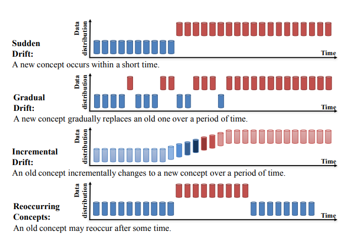![](https://images.datacamp.com/image/upload/v1673459876/Concept_Drift_b16df50c98.png){fig-alt="Four different types of data drift described visually." fig-align="center"}

::: aside
Image taken from [DataCamp](https://www.datacamp.com/tutorial/understanding-data-drift-model-drift).
:::

## Cognitive biases 

Cognitive biases are systematic patterns of deviation from norm and/or rationality in judgment. They are often studied in psychology, sociology and behavioral economics.^[Haselton MG, Nettle D, Andrews PW (2005). "The evolution of cognitive bias" (PDF). In Buss DM (ed.). The Handbook of Evolutionary Psychology. Hoboken, NJ: John Wiley & Sons Inc. pp. 724–746.]

Some biases to be aware of:

- **Survivorship bias**: Analyzing just the data that is available without analyzing the larger situation.
- **False causality**: Seeing correlation between two variables does not imply one causes the other to occur. ^[Something fun to explore: [Spurious correlations](https://www.tylervigen.com/spurious-correlations)]
- **Availability bias**: Drawing conclusions on limited data. 
- **Confirmation bias**: Manipulating data to confirm your own hypothesis. 

## Simpson's paradox 

Simpson's paradox occurs when groups of data show one particular trend, but this trend is reversed when the groups are combined together. Understanding and identifying this paradox is important for correctly interpreting data. ^[Simpson, Edward H. (1951). "The Interpretation of Interaction in Contingency Tables". Journal of the Royal Statistical Society, Series B. 13: 238–241.]

:::: {.columns}

::: {.column width="50%"}

<br>

A baseball player can have higher batting average than another on each of two years, but lower than the other when the two are combined. In one case, David Justice had a higher batting average than Derek Jeter in 1995 and 1996, but across the two years, Jeter's average was higher. ^[[Simpon's Paradox by Brilliant](https://brilliant.org/wiki/simpsons-paradox)]

:::

::: {.column width="50%" layout-valign="top"}

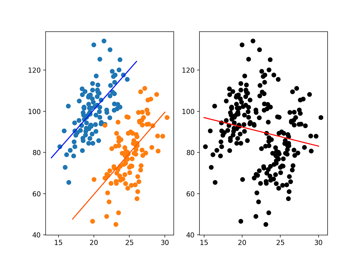![](https://miro.medium.com/v2/resize:fit:1400/1*HDi8HuaVrumdFP-W9e4PtA.png){fig-alt="Picture explaining Simpson's paradox." fig-align="center"}

:::

::::

## Goodhart's law 

:::: {.columns}

::: {.column width="50%"}

_Any observed statistical regularity will tend to collapse once pressure is placed upon it for control purposes._ ^[Goodhart, Charles (1975). "Problems of Monetary Management: The U.K. Experience". In Courakis, Anthony S. (ed.). Inflation, Depression, and Economic Policy in the West. Totowa, New Jersey: Barnes and Noble Books (published 1981). p. 116. ISBN 0-389-20144-8.]

<br><br>

or a better way of putting it is: 

<br><br>

**When a measure becomes a target, it ceases to be a good measure.** ^[Strathern, Marilyn (1997). "'Improving ratings': audit in the British University system". European Review. John Wiley & Sons. 5 (3): 305–321.]

:::

::: {.column width="50%"}

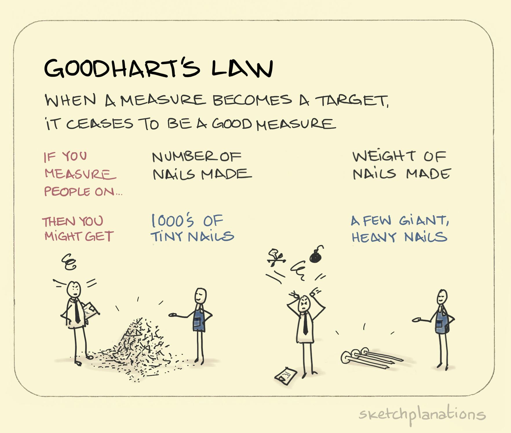![](https://images.prismic.io/sketchplanations/6336f4c3-4c89-41f6-998f-ac595fb33a66_167369765942.jpg?auto=compress%2Cformat&fit=max&w=3840&q=50){fig-align="center" fig-alt="Sketchplanations cartoon explaining Goodhart's Law"}

:::

::::

# Sharing your data with others

## Reproducibility and Replicability 

:::: {.columns}

::: {.column width="75%"}
Reproducibility is the ability of independent investigators to draw the same conclusions from an experiment by following the documentation shared by the original investigators. Hence, reproducibility requires that another, independent team of investigators have to conduct the same experiment. ^[Gundersen Odd Erik. 2021. The fundamental principles of reproducibility. _Phil. Trans. R. Soc. A._ 379: 20200210. http://doi.org/10.1098/rsta.2020.0210]

Easy tips for enabling others to reproduce your work:

:::: {.columns id="small-bullets"}

::: {.column width="50%"}

- Use a static random seed
  - in R: `set.seed(42)`
  - in Python: `random.seed(42)`
- Document your environment
  - in R: `library(renv)`
  - in Python: `pip freeze > requirements.txt`

:::

::: {.column width="40%"}

- Use version control (e.g., Github, Bitbucket)
- Use notebooks
  - in R: [R Markdown](https://rmarkdown.rstudio.com/)
  - in Python: [Jupyter](https://jupyter.org/)
  - in either: [Quarto](https://quarto.org/)

:::

::::

:::

::: {.column width="25%"}
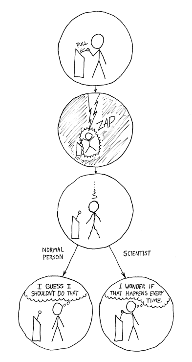![](https://imgs.xkcd.com/comics/the_difference.png){fig-align="center" height="50%"}^[[xkcd 242](https://xkcd.com/242/)]
:::

::::

## Using pins

The pins package publishes data, models, and other R objects, making it easy to share them across projects and with your colleagues. You can pin objects to a variety of pin boards, including:

- folders (to share on a networked drive or with services like DropBox)
- Posit Connect
- Amazon S3
- Google Cloud Storage
- Azure storage
- Microsoft 365 (OneDrive and SharePoint). 

Pins can be automatically versioned, making it straightforward to track changes, re-run analyses on historical data, and undo mistakes.^[https://pins.rstudio.com/] Pins is available in [R](https://pins.rstudio.com/) and [Python](https://rstudio.github.io/pins-python/).

## Discussion / Contact Info

<br><br>

::: {id="credit"}

### Christopher Teixeira

[christopherteixeira.com](https://www.christopherteixeira.com)

:::

:::: {.columns}

::: {.column width="40%"}

<br><br>

[{{< fa envelope size=xl >}} chris@christopherteixeira.com](mailto:chris@christopherteixeira.com)

[{{< fa brands linkedin size=xl >}} in/christopherteixeira](https://www.linkedin.com/in/christopherteixeira/)

[{{< fa brands github size=xl >}} ct-analytics](https://github.com/ct-analytics)

:::

::: {.column width="60%"}

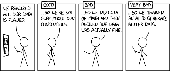![](https://imgs.xkcd.com/comics/flawed_data.png){fig-align="center"}

:::

::::

::: aside
[xkcd 2494](https://xkcd.com/2494/)
:::